Horizon computation#
The horizon of a given detector is the maximum (luminosity) distance at which it can see a certain kind of signal.
Recall that a gravitational waveform at cosmological distances can be computed by replacing the \(1/r\) prefactor with \(1/d_L\), where \(d_L\) is the luminosity distance, and by mapping the masses \(m_i \to (1+z) m_i\), where \(z\) is the redshift. For details on this and a derivation, see section 4.1.4 of Maggiore (2007).
Therefore, if we fix the signal, computing the horizon is just a matter of finding a solution to
where \(\text{SNR}^*\) is some minimum-detection threshold (on the order of 9), and also where a relation between \(z\) and \(d_L\) is assumed — by default, we might choose a FLRW cosmology with the latest Planck parameters, for example.
The \(z\) dependence means the relation is not as simple as \(\text{SNR} \sim 1 / d_L\), as we would expect at low redshift. Specifically, the source-frame masses get redshifted, which shifts the signal to lower frequencies.
An example of how the SNR curve against distance can look is the following:
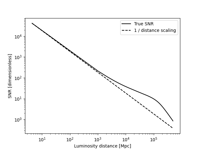
SNR as a function of luminosity distance for a \(10^3 + 10^3\) solar mass BH binary, as seen by LGWA.#
The SNR being higher than the \(1/d_L\) scaling is due to the fact that the signal’s amplitude increases with the mass, which is effectively increased due to the redshift.
Note, however, that this is not a general fact: the redshifting also means that the signal might end inside the detector band or before it, thereby reducing the SNR.
In general, though, the equation given above is nonlinear and needs to be solved numerically.
This is accomplished by the GWFish.modules.horizon function.